Bell's Inequalities: A quantum computing experiment with Qiskit
1. Introduction
1.1. Intro to the intro
I’m not quite sure what this article is—a mix of coding experiment, science communication, and maybe just a fun project for someone who in another life would have wanted to be a physicist.
I’ve had this in my drawer for a while, since I read this article by some CERN researchers that explains how you can simulate an experiment on Bell’s inequalities using the Qibo framework.
Reading that article led me to a realization that, at least for me, is super fascinating: today in 2025, anyone with even basic programming knowledge and a couple of foundational concepts can run (or at least simulate) a quantum mechanics experiment that 20 or 30 years ago would only have been possible in a physics lab with extremely expensive equipment.
However, just copy-pasting code and running it doesn’t seem particularly interesting to me, at least not without really understanding what we’re talking about. That’s why I started studying a bit of the history and some basic principles.
This little deep-dive exercise, which spans more than a century of history—from the origins (1905) to the 2022 Nobel Prize (in my opinion, it deserves a movie or a novel)—and touches on some of the deepest epistemological problems humanity has ever faced, has given meaning to the final exercise, which still remains little more than copy-paste from the CERN article and some suggestions from Claude 😃
1.2. The real intro
Many people wonder if/when quantum computing will become a reality. To be honest, after strong market expansion in the post-COVID period, there was a moderate growth trend between 2022 and 2024, probably due to the global economic crisis and attention shifting to generative artificial intelligence.
| Year | Global Market Revenues |
|---|---|
| 2020 | ████████ $412M |
| 2021 | ████████ $391M |
| 2022 | ██████████████ $713M |
| 2023 | █████████████████ $885M |
| 2024 | ███████████████████████ $1,107M |
Sources:
In particular, in 2024 the main players operating in the Quantum Computing sector slowed down a bit in the race for more qubits, focusing on developing new architectures to reduce the so-called quantum decoherence phenomenon, which is one of the main obstacles to the scalability of current systems. However, in 2025 there’s been a resurgence, with announcements of new prototypes from IBM, Google, and Microsoft, and in the last 6 months, Rigetti’s stock (another player that, unlike the previous ones, operates exclusively in the quantum computing sector) has grown by 380% on the stock market!
In any case, we haven’t yet seen any real revolution, and almost everyone agrees that QC will probably never replace the classical computing model but, at best, will complement it, allowing for efficient solutions to complex problems.
An example of a problem that could be efficiently solved with a quantum computer is the factorization of very large integers into prime factors, using Shor’s algorithm to evolve (or break) currently used cryptographic systems.
However, current limitations of quantum computers don’t yet allow for the efficient execution of this algorithm on numbers large enough to undermine the security of current cryptographic systems. Apart from this potential use case and some other special cases limited to very specific fields—such as Grover’s algorithm for searching in unsorted lists—we still don’t see practical applications of quantum computing. While we wait for practical applications to arrive, we can already today use it to conduct real quantum mechanics experiments. These experiments, which for me are little more than a game, refer to much more serious work that lasted several decades and led John Clauser, Alain Aspect, and Anton Zeilinger to win the 2022 Nobel Prize in Physics: experiments on Bell’s Inequalities.
Needless to say, what’s reported here isn’t even a real “experiment,” since I used a simulator (not a real quantum computer). Moreover, the circuit I implemented is based on an extreme simplification of the original experiment, but the theoretical principles are the same, and it could be ported to a real commercial Quantum Computer with little effort. So it’s an interesting exercise to understand what “non-locality” really means in quantum mechanics and how the same principles underlie the functioning of Quantum Computing.
To do this, we need a few ingredients:
- A bit of history
- Some notions of quantum mechanics
- A deep dive into Bell’s inequalities
- The basics of Quantum Computing
2. A bit of history
2.1. Einstein and quantum mechanics
Perhaps not everyone knows that Albert Einstein didn’t win the Nobel Prize for his theories on relativity, but rather for his explanation of the photoelectric effect, drawing from an idea by Max Planck. Like his studies on relativity, that work by Einstein was enormously important for 20th-century physics because it kicked off the other great branch of physics: quantum mechanics. A noteworthy fact is that no Nobel Prize has ever been awarded for discoveries directly connected to the theory of relativity, while since 1920, at least 16 Nobels have been awarded for studies or discoveries directly connected to quantum mechanics.
At the beginning of the twentieth century, the idea of light as a “corpuscle” was in contrast with the wave representation of light, which was well established and dated back to the works of Christiaan Huygens from around the mid-1600s. Over the centuries, the wave nature was questioned several times, but interference experiments and the solid theoretical foundations introduced by Thomas Young in 1801, and later by James Clerk Maxwell with his electromagnetic theory of light, seemed to have definitively closed the question. Consequently, Planck himself, when he introduced the idea of quanta in 1900, didn’t really believe in the corpuscular nature of light. From his point of view, it was just a theoretical abstraction that served to explain the problem of black body radiation, but had no real physical correspondence.
Einstein’s great merit was taking Planck’s intuition seriously—that energy couldn’t be exchanged continuously but rather in discrete “packets” that Planck called “quanta” (hence the name “quantum mechanics”). In 1905, Einstein applied this idea to explain the photoelectric effect, hypothesizing that light was composed of “light quanta,” which we now call photons, and this earned him the Nobel Prize in Physics in 1921.
However, initially no one believed Einstein, not even Max Planck, who had provided the initial intuition. It was only thanks to the work of Robert Millikan—who, with the objective of discrediting Einstein’s thesis, conducted numerous experiments and took several years to surrender to the fact that Einstein’s explanation of the photoelectric effect was correct and thus the hypothesis of quanta was anything but a simple theoretical abstraction.
From here on, it’s a succession of studies and discoveries that make quantum mechanics the most accurate and precise physical theory ever developed, leading in just a few years to an incredible sequence of Nobel Prizes, among which the most important are:
- 1922 - Niels Bohr for his studies on atomic structure
- 1923 - Millikan for his experimental work on the photoelectric effect and the measurement of electron charge
- 1927 - Arthur Compton for the discovery of the Compton effect
- 1929 - Louis de Broglie for the discovery of the wave nature of the electron
- 1932 - Werner Heisenberg for the formulation of quantum mechanics
- 1933 - Erwin Schrödinger and Paul Dirac for the formulation of wave mechanics
- 1945 - Wolfgang Pauli for the discovery of the exclusion principle
- 1954 - Max Born for the formulation of quantum mechanics in probabilistic terms
- 1965 - Richard Feynman, Julian Schwinger, and Sin-itiro Tomonaga for the development of quantum electrodynamics
Ironically, Einstein himself—who had started that revolution—became increasingly skeptical of the theory as it developed, to the point of isolating himself from the scientific community that had meanwhile fully embraced it.
But why was Einstein so skeptical about the representation of reality according to quantum mechanics? The answer to this question has to do with the very concept of Reality itself and requires a deeper look to understand Einstein’s point of view.
2.2. What is reality?
In a certain sense, Einstein’s approach to the problems raised by quantum mechanics was similar to what had characterized his approach to Relativity. When he faced an apparently unsolvable problem (such as the constancy of the speed of light across all inertial reference frames), he didn’t try at all costs to adapt the theory, but rather began to question and define a new formalism for concepts that seemed well established, such as the concept of simultaneity, time, and space.
Something similar happened with the concept of Reality, through which Einstein, Podolsky, and Rosen formulated the famous EPR paradox, which questioned the completeness of quantum mechanics.
From Einstein’s point of view, the description of the physical world had to obey 2 fundamental principles:
- Locality: an object can only be influenced by its immediate surroundings, and not by events occurring at arbitrarily large distances. In other words, there cannot be “action at a distance” (spooky action at a distance).
- Realism: objects have defined properties independent of observation. In other words, reality exists independently of whether we observe it or not.
The EPR Paradox describes some thought experiments through which the authors try to demonstrate that quantum mechanics cannot be a complete theory because it violates at least one of the principles listed above.
In other words, if quantum mechanics is correct, then at least one of the following statements holds:
- the principle of locality is false, and therefore there exist actions at a distance that violate the speed of light limit
- the principle of realism is false, and therefore objects don’t have defined properties independent of observation, but rather physical properties manifest only at the moment they are measured
From a technical point of view, the EPR paradox is based on the concept of entanglement which, besides being one of the strangest and most fascinating concepts in quantum mechanics (often misunderstood and misinterpreted), is also at the basis of how quantum computers work.
2.3 The scientific world’s interest in the question
For decades, the entire question of the EPR paradox and the epistemological interpretation of quantum mechanics remained confined to philosophical discussions among a few experts, and already after the 1930s, quantum mechanics was so well established that no one worried about these aspects anymore. Bell himself worked as a particle physicist at various research institutions in the UK and then at CERN and devoted himself to this topic only in his spare time. In 1964, during a sabbatical year in the United States, Bell published the famous article “On the Einstein Podolsky Rosen paradox” in which he proposed a way to experimentally verify whether Einstein was right or not. The article aroused some interest, but nevertheless, even after Bell’s publication, only a few daring souls were interested in a potential experiment to verify Bell’s inequalities, also because shortly after, the very journal in which Bell had published the article went bankrupt, and this certainly didn’t help spread the idea.
John Clauser himself, one of the three 2022 Nobel Prize winners, was initially not very convinced about tackling the question and recounts that when he asked the legendary Richard Feynman for advice about doing his first experiment to test Bell’s inequalities, he was told it was a “waste of time” because quantum mechanics had already been extensively verified and no one expected Einstein to be right.
3. Some notions of quantum mechanics
3.1. Quantum superposition
In quantum mechanics, a system can be in a state of superposition, that is, in a combination of multiple states simultaneously.
In the world of quantum computing, the superposition state can be implemented through the application of some operators (quantum gates) on qubits, the quantum analog of the classical bit. While a classical bit can only take values 0 or 1, a qubit can be in a superposition of the two states, represented mathematically as:
$$|\psi\rangle = \alpha|0\rangle + \beta|1\rangle$$where $\alpha$ and $\beta$ are complex numbers that satisfy the condition $|\alpha|^2 + |\beta|^2 = 1$ .
3.2. Quantum measurement
When we measure a qubit, the superposition “collapses” into one of the two basis states (0 or 1), with probabilities $|\alpha|^2$ and $|\beta|^2$ respectively.
This is one of the most controversial aspects of quantum mechanics: before measurement, the system is effectively in both states simultaneously (according to the Copenhagen interpretation), but the moment we measure it, reality “chooses” one of the two states probabilistically.
Einstein never accepted this interpretation. At first, he tried to demonstrate that quantum mechanics was incorrect. His criticisms of Bohr during the Solvay Conferences and the thought experiments that tried to challenge the theoretical framework of quantum mechanics that we can now call “orthodox” are now legendary. However, Bohr and Heisenberg always managed to find an answer to Einstein’s challenge, supported by the theory itself. In the end, Einstein surrendered to the evidence: quantum mechanics was correct.
However, he continued to maintain that it was an incomplete theory and that there had to be a more complete description of reality that included “hidden variables” that would allow predicting the measurement result deterministically.
Beyond the philosophical implications, the concept of “measurement” also has practical implications in quantum programming since, for example, we can’t simply “read” the state of a qubit in a superposition state without altering it. In the Copenhagen interpretation, this alteration (that is, this “measurement”) is equivalent to the concept of wave function collapse.
3.3. Entanglement
Entanglement (quantum correlation) is perhaps the strangest and most counterintuitive phenomenon in quantum mechanics. When two particles are entangled, they form a single quantum system, even if they are separated by arbitrarily large distances.
This correlation leads to phenomena that Einstein called “spooky actions at a distance” and led him to believe that quantum mechanics must be an incomplete theory.
Nevertheless, as strange and counterintuitive as it is (in fact, perhaps precisely because of this aspect), the phenomenon of entanglement has been experimented and verified countless times in laboratories.
In the vast majority of cases, tests refer to individual particles, but there are also cases where the entangled state of macroscopic systems like molecules has been verified.
The most extreme and famous example is the thought experiment of Schrödinger’s cat, which is simultaneously alive and dead until it’s observed.
3.3.1. Entanglement and Quantum Computing
From the Quantum Computing perspective, a classic example is that of two qubits in a Bell state:
$$|\Phi^+\rangle = \frac{1}{\sqrt{2}}(|00\rangle + |11\rangle)$$This state represents a superposition in which the two qubits are both 0 or both 1 with 50% probability. The extraordinary thing is that when we measure the first qubit and obtain (for example) 0, instantly the second qubit also collapses to state 0, regardless of the distance separating them.
3.4 Hidden variable theories
According to Einstein, quantum mechanics was an incomplete theory: the probabilities we observe in quantum measurements wouldn’t reflect a real indeterminacy of nature, but simply our ignorance of some hidden variables that in theory could be used to precisely determine the measurement result.
To better understand this concept, we can make an analogy with flipping a coin:
- From a practical point of view, the result (heads or tails) seems random with 50% probability
- But we know that in reality the result is completely determined by initial conditions: speed, launch angle, force, air resistance, etc.
- If we perfectly knew all these “hidden variables,” we could predict the result with certainty
Einstein believed something similar happened in quantum mechanics. When we prepare an electron in a superposition state and then measure it, according to Einstein:
- The electron already possesses a defined property before the measurement
- This property is determined by variables that the current theory doesn’t include (hidden variables)
- The probabilistic nature of quantum mechanics derives only from our ignorance of these variables
- A more complete theory that included these variables would be completely deterministic
This point of view is called local realism with hidden variables:
- Local: hidden variables are intrinsic properties of the system, not influenced by distant events
- Realist: physical properties exist independently of observation
- Deterministic: knowing the hidden variables, the measurement result would be predetermined
The EPR paradox was precisely an attempt by Einstein, Podolsky, and Rosen to demonstrate that such hidden variables must necessarily exist to maintain the principles of locality and realism.
4. A deep dive into Bell’s inequalities
4.1. John Bell’s work
In 1964, Irish physicist John Stewart Bell proposed a way to experimentally verify whether Einstein was right. Bell formulated a series of mathematical inequalities that must be satisfied if the principle of local realism holds (that is, if both the principle of locality and that of realism hold together).
Bell’s brilliant idea was to find a measurable quantity that:
- If quantum mechanics is correct, violates the inequalities
- If there exists a “local hidden variables” theory (as Einstein maintained), respects the inequalities
This work, however, was entirely mathematical in nature. The brilliance of the physicists who came after (and for which the 2022 Nobel was ultimately recognized) was to design and carry out experiments to implement it in the real world.
4.2. The CHSH test
One of the most used formulations of Bell’s inequalities is the CHSH test (from Clauser, Horne, Shimony, and Holt), which takes its name from the four physicists who proposed it in 1969.
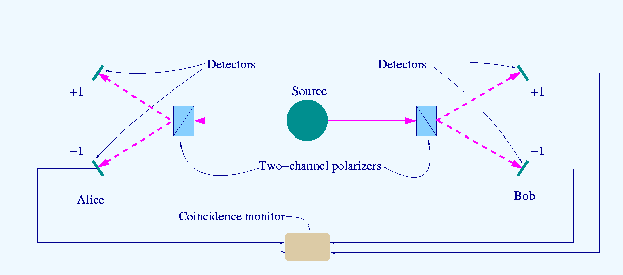
The experiment involves:
- A source that produces entangled particle pairs (for example, polarized photons)
- The usual “Alice” and “Bob” from all physics experiments, who can choose between two possible measurements to perform
- Measuring the correlations between the results obtained by Alice and Bob
More formally:
- Alice can choose to measure according to angle $a_0$ or $a_1$
- Bob can choose to measure according to angle $b_0$ or $b_1$
- Each measurement produces a result +1 or -1
The CHSH quantity is then defined:
$$S = E(a_0, b_0) + E(a_0, b_1) + E(a_1, b_0) - E(a_1, b_1)$$where $E(a_i, b_j)$ is the correlation between Alice’s and Bob’s measurements.
4.2.1. Non-commutative quantities
In the CHSH test, Alice and Bob measure photon polarization according to different angles, but similar experiments can be done with other physical quantities, such as the spin of electrons (also in an entangled state).
In any case, the experiment only works if the measured quantities are of a non-commutative nature.
In classical physics, if we want to measure two properties of an object (for example, its position and its velocity), we can do so in any order and always get the same results. The order of measurements doesn’t matter.
In quantum mechanics, however, there exist pairs of physical quantities for which the order of measurements is important. When we measure A first and then B, we get different results compared to when we measure B first and then A. Mathematically, this is expressed by saying that the corresponding operators don’t commute:
$$\hat{A}\hat{B} \neq \hat{B}\hat{A}$$Non-commutativity is closely linked to Heisenberg’s uncertainty principle.
The most famous examples of non-commutative quantities are:
- Position and momentum: Heisenberg’s uncertainty principle derives precisely from the non-commutativity of these two quantities
- Spin components along different axes: measuring spin along the x-axis and then along the y-axis gives different results compared to the inverse order
- Photon polarization according to different angles: precisely what we measure in the CHSH test
In our experiment, when Alice measures polarization according to angle $a_0 = 0°$ and Bob according to $b_0 = 45°$ , they are measuring non-commutative quantities because they’re associated with the same entangled system.
Source: wikipedia
According to “orthodox” quantum mechanics, we can summarize that:
- We cannot simultaneously know both polarizations with absolute certainty
- The first measurement influences the second: if Alice measures first, Bob’s result will be influenced by the wave function collapse caused by Alice’s measurement
- There are no “pre-existing values” for both polarizations: properties manifest only at the moment of measurement
Conversely, hidden variable theories assume that each particle carries a “hidden instruction” that predetermines the result for every possible measurement angle. But if quantities don’t commute, there cannot simultaneously exist predetermined values for all possible measurements.
Bell’s genius was realizing that this difference between the classical world (where all quantities commute) and the quantum one (where some quantities don’t commute) translates into a measurable difference in statistical correlations over a sufficiently large sample of measurements.
- According to local realism: $|S| \leq 2$
- According to quantum mechanics: $|S|$ can reach up to $2\sqrt{2} \approx 2.828$
But why these limits? Let’s try to understand with an intuitive analogy.
4.2.1.1. The local realism reasoning (the limit of 2)
Imagine that each pair of entangled particles carries a hidden “instruction sheet” that predetermines the result for every possible measurement angle. This sheet contains 4 predetermined values:
- $A_0$ : Alice’s result if measuring according to $a_0$ (can be +1 or -1)
- $A_1$ : Alice’s result if measuring according to $a_1$ (can be +1 or -1)
- $B_0$ : Bob’s result if measuring according to $b_0$ (can be +1 or -1)
- $B_1$ : Bob’s result if measuring according to $b_1$ (can be +1 or -1)
For each single pair of particles, we can calculate:
$$S_{\text{single}} = A_0 B_0 + A_0 B_1 + A_1 B_0 - A_1 B_1$$Let’s do a concrete example. Suppose a particular pair has:
- $A_0 = +1$ , $A_1 = -1$ , $B_0 = +1$ , $B_1 = +1$
Then:
$$S = (+1)(+1) + (+1)(+1) + (-1)(+1) - (-1)(+1) = 1 + 1 - 1 + 1 = 2$$Let’s try another combination:
- $A_0 = +1$ , $A_1 = +1$ , $B_0 = +1$ , $B_1 = -1$
We can rewrite $S$ as:
$$S = A_0(B_0 + B_1) + A_1(B_0 - B_1)$$Now observe that:
- If $B_0 = B_1$ , then $(B_0 + B_1) = \pm 2$ and $(B_0 - B_1) = 0$ , so $S = \pm 2A_0$ , i.e., $|S| = 2$
- If $B_0 = -B_1$ , then $(B_0 + B_1) = 0$ and $(B_0 - B_1) = \pm 2$ , so $S = \pm 2A_1$ , i.e., $|S| = 2$
In both cases, for a single pair with predetermined values, we always get $|S| = 2$
When we make many measurements and calculate the average of the correlations $E(a_i, b_j)$ , we’re averaging over all possible combinations of hidden instructions. But since each single pair gives $|S| = 2$ , the average can never exceed this value:
$$|S| = |E(a_0, b_0) + E(a_0, b_1) + E(a_1, b_0) - E(a_1, b_1)| \leq 2$$This is therefore the classical limit and is valid for any local hidden variable theory.
4.2.1.2. The quantum reasoning (the limit of 2√2)
In quantum mechanics, instead, predetermined values don’t exist. The particles are in an entangled Bell state:
$$|\Phi^+\rangle = \frac{1}{\sqrt{2}}(|00\rangle + |11\rangle)$$When Alice and Bob measure according to different angles, the correlations depend on the angular difference $\theta$ between their measurement directions according to the formula:
$$E(\theta) = \cos(2\theta)$$For the optimal angles of the CHSH test:
- $a_0 = 0°$ , $a_1 = 45°$
- $b_0 = 22.5°$ , $b_1 = -22.5°$
With these angles:
- $E(a_0, b_0) = \cos(2 \times 22.5°) = \cos(45°) = \frac{1}{\sqrt{2}}$
- $E(a_0, b_1) = \cos(2 \times 22.5°) = \cos(45°) = \frac{1}{\sqrt{2}}$
- $E(a_1, b_0) = \cos(2 \times 22.5°) = \cos(45°) = \frac{1}{\sqrt{2}}$
- $E(a_1, b_1) = \cos(2 \times 67.5°) = \cos(135°) = -\frac{1}{\sqrt{2}}$
Therefore:
$$S = \frac{1}{\sqrt{2}} + \frac{1}{\sqrt{2}} + \frac{1}{\sqrt{2}} - \left(-\frac{1}{\sqrt{2}}\right) = \frac{4}{\sqrt{2}} = 2\sqrt{2} \approx 2.828$$This instead is Tsirelson’s bound and is the maximum theoretical value predicted by quantum mechanics.
4.2.1.3. Where does this difference come from?
The fundamental difference is this:
Local realism: assumes that each particle has 4 defined properties simultaneously ($A_0, A_1, B_0, B_1$ ), even if we only measure one. This assumption limits the possible correlations.
Quantum mechanics: properties don’t exist before measurement. Particles are in superposition and the measurement angle determines the “basis” onto which we project the state. This allows stronger correlations.
An analogy: it’s as if in the classical case each particle carried with it 4 already-flipped coins (but covered), while in the quantum case the coins are flipped only when we uncover them, and the way we uncover Alice’s instantly influences the probabilities for Bob’s, even if they’re far apart.
4.3. The experiments that earned the 2022 Nobel
Starting from the 1970s, a series of experiments based on Bell’s theoretical framework and particularly on the CHSH test unequivocally demonstrated that Bell’s inequalities are violated exactly as predicted by the theoretical framework of quantum mechanics, confirming that local realism cannot be maintained:
- 1972 - John Clauser: first experiment that violated Bell’s inequalities using polarized photons
- 1982 - Alain Aspect: more refined experiments that eliminated various possible “loopholes”
- 1998-2015 - Anton Zeilinger: experiments with entanglement over increasingly greater distances, eventually demonstrating quantum teleportation
In 2022, these three physicists received the Nobel Prize in Physics precisely for these pioneering experiments.
4.3.1. The “loopholes” and how they were eliminated
Despite Clauser’s first experiments in the 1970s having violated Bell’s inequalities, some possible technical objections remained that could have allowed a supporter of local realism to doubt the results. These objections are called loopholes, and much of the subsequent experimental work focused on eliminating them one by one.
4.3.1.1. Locality Loophole
The problem: In the first experiments, Alice’s and Bob’s measurements weren’t sufficiently separated in spacetime. In theory, a classical signal (traveling at or below the speed of light) could have traveled from one detector to the other, influencing the result without the experimental apparatus being able to detect it.
Alain Aspect’s solution (1982): Aspect introduced a system of ultrafast switching of measurement angles:
- Measurement angles were randomly changed during photon flight
- The change occurred so quickly that no subluminal signal could travel from one detector to the other
- This guaranteed the spacelike separation of measurements
These modifications were implemented so that the time interval between production and detection was 20 ns, while the channel switches inverted orientation asynchronously every 10 ns, keeping the various sections sufficiently far apart to guarantee spacelike distances between them. This ensures that Alice’s measurement event is causally disconnected from Bob’s.
4.3.1.2. Fair Sampling Loophole
The problem: No detector is 100% perfect. In early photon experiments, only a small fraction of produced particle pairs was actually detected and measured. In Clauser’s experiments, for example, detection efficiency was less than 5%.
This opens up a possible objection: how can we be sure that the particle pairs actually detected are a representative sample of all pairs produced?
A supporter of local realism could argue that:
- Particles carry “hidden instructions” that determine both the measurement result and the probability of being detected
- Particles with certain combinations of hidden instructions have a higher probability of being detected than others
- The observed sample is therefore biased, and measured correlations don’t reflect the true correlations of the complete set
In other words, it’s as if we did a political poll by only interviewing people who answer the phone: the sample might not be representative of the general population.
Mathematically, this objection works because the proof of Bell’s Inequalities assumes all produced pairs are measured. If we can only measure a subset, and this subset isn’t randomly chosen but depends on hidden variables, then the inequalities could be violated even in a local hidden variable theory.
The fair sampling assumption: For many years, experiments relied on the fair sampling assumption, which assumes that detected particles are a representative random sample. This assumption is reasonable from a physics standpoint, but it’s not a rigorous proof.
The solution: To completely eliminate this loophole, you need to achieve detection efficiency above a critical threshold. For the CHSH test, this threshold is about 82.8% (more precisely, $\eta > 2/3 \approx 66.7\%$ for optimal configurations, but in practice you need higher efficiency to account for other factors).
This goal was very difficult to achieve and required decades of technological progress:
First solution - Trapped ions (2000s):
- Ions (charged atoms trapped in electromagnetic fields) are much more controllable than photons
- They can be kept in precise positions and measured with very high efficiency (>90%)
- Pioneering experiments by Rowe et al. (2001) and Matsukevich et al. (2008) achieved efficiencies above the critical threshold
- Disadvantage: ions are difficult to spatially separate, making it more complicated to simultaneously close the locality loophole
Second solution - Superconducting detectors for photons (2010s):
- Superconducting nanowire single-photon detectors (SNSPDs) revolutionized photon detection
- They operate at cryogenic temperatures (near absolute zero)
- They achieve 75-98% efficiency in the infrared band
- They allow using photons (easily separable over large distances) while maintaining high detection efficiency
Third solution - Neutral atoms and color centers:
- Color centers in diamond (like NV centers - nitrogen-vacancy): defects in the diamond crystal structure that behave like single quantum systems
- Trapped neutral atoms: atoms cooled with lasers and trapped in optical tweezers
- Combine the advantages of both approaches: high efficiency and possibility of spatial separation
4.3.1.3. Freedom-of-Choice Loophole
The problem: How are measurement angles chosen for Alice and Bob? If the choice isn’t truly random but is somehow correlated with the particles’ “hidden instructions,” then the results could be explained with local realism.
This objection may seem strange, but from a logical point of view it’s valid: if the universe is deterministic, then even the “random” choice of angle could be predetermined by the same hidden variables that determine the measurement result!
The solution: Use sources of randomness that are as “free” as possible:
Quantum random number generators (QRNG): exploit intrinsically random quantum processes
Light from distant stars (Zeilinger’s experiments, 2017): they used light coming from stars thousands of light-years away to decide measurement angles. This way, the “hidden instructions” would have had to be correlated with events that, at least as a first approximation, we can assume to be causally disconnected from the entangled particles.
Human participation: in an experiment called “The BIG Bell Test” (2016), thousands of people around the world chose measurement angles through an online video game
4.3.1.4. Memory Loophole
The problem: If particle pairs are measured in sequence and results are accumulated over time, there could be spurious correlations due to variations in the experimental apparatus.
The solution: Ensure the apparatus is stable over time or, even better, complete the experiment in such a short time as to exclude instrumental drift.
4.3.1.5. “Loophole-free” experiments
The real milestone was reached in 2015, when three independent groups succeeded in carrying out experiments that closed simultaneously all the main loopholes:
Delft (Netherlands) - Hensen et al.: used two color centers in diamond (defects in the crystal structure) separated by 1.3 km, connected via entanglement
- ✓ Locality loophole closed (distance 1.3 km)
- ✓ Detection loophole closed (efficiency > 90%)
Vienna (Austria) - Giustina et al.: used entangled photons with superconducting detectors
- ✓ Locality loophole closed
- ✓ Detection loophole closed (75% efficiency)
Boulder, Colorado (USA) - Shalm et al.: used entangled photons separated by 185 meters
- ✓ Locality loophole closed
- ✓ Detection loophole closed (75% efficiency)
These experiments definitively demonstrated that it’s not possible to save local realism: nature truly violates Bell’s inequalities, and it’s not an experimental artifact.
4.3.1.6. Are there still open loopholes?
From a practical point of view, no: modern experiments are convincing beyond any reasonable doubt. However, from a philosophical point of view, there still exists an extremely speculative theoretical “loophole”:
This is the so-called Superdeterminism: the hypothesis that everything in the universe is predetermined from the Big Bang, including experimenters’ choices and measurement results. In this extreme scenario, free will wouldn’t exist even in an operational sense. This position is considered by most physicists to be a non-falsifiable hypothesis and therefore not scientific.
In conclusion, scientific consensus is unanimous: Bell’s inequalities are violated, local realism is incompatible with nature, and the experiments that demonstrated it fully deserved the 2022 Nobel Prize.
5. The basics of Quantum Computing
5.1. Qubits and quantum gates
In quantum computing, information is encoded in qubits instead of classical bits. Qubits can be physically implemented in various ways: electron spin, polarized photons, energy states of trapped atoms, etc.
Operations on qubits are performed through quantum gates, which are the analog of classical logic gates (AND, OR, NOT, etc.). The most common quantum gates are:
- X gate: similar to classical NOT, swaps states |0⟩ and |1⟩
- H gate (Hadamard): creates an equiprobable superposition between |0⟩ and |1⟩
- CNOT gate: two-qubit gate that inverts the second qubit if the first is |1⟩
- Rotation gates: allow manipulating the qubit state with precision
5.2. Quantum circuits
A quantum program is represented as a quantum circuit, a sequence of quantum gates applied to one or more qubits. Unlike classical circuits, quantum circuits are reversible (except for measurement, which is irreversible).
To create entanglement between two qubits, typically a combination of Hadamard and CNOT gates is used:
- Apply an H gate to the first qubit to create superposition
- Apply a CNOT gate using the first qubit as control and the second as target
This creates a Bell state, completely entangled.
q0: ──H──■──
         │
q1: ─────X──
5.3. Quantum Computing platforms
Today there are several platforms that allow running real programs on actual quantum computers, including for example:
- IBM Quantum Experience: allows free access to IBM’s real quantum computers
- Amazon Braket: AWS’s quantum computing service
- Google Quantum AI: Google’s quantum computing platform
- Local simulators: libraries like Qiskit, Cirq, Q# allow simulating quantum circuits on your own computer
6. Let’s do the experiment
6.1. Experiment setup
We can reproduce the CHSH test using a real quantum computer or a simulator. We’ll use two qubits in an entangled state and measure correlations according to different configurations.
Necessary ingredients:
- A quantum computing platform (Qiskit, IBM Quantum, etc.)
- Two qubits
- Quantum circuits to create entanglement and perform rotations
6.2. The quantum circuit
The basic circuit for the CHSH test is as follows:
from qiskit import QuantumCircuit, QuantumRegister, ClassicalRegister

# Create 2 qubits and 2 classical bits for measurements
qr = QuantumRegister(2, 'q')
cr = ClassicalRegister(2, 'c')
qc = QuantumCircuit(qr, cr)

# Step 1: Create an entangled Bell state
qc.h(qr[0])        # Hadamard on first qubit
qc.cx(qr[0], qr[1]) # CNOT to create entanglement

# Step 2: Apply rotations for Alice and Bob
# (angles depend on which configuration we want to test)
qc.ry(theta_a, qr[0])  # Rotation for Alice
qc.ry(theta_b, qr[1])  # Rotation for Bob

# Step 3: Measure
qc.measure(qr, cr)
For the optimal CHSH test, the angles must be:
- $a_0 = 0°$ , $a_1 = 45°$ (for Alice)
- $b_0 = 22.5°$ , $b_1 = -22.5°$ (for Bob)
6.3. Complete code
from qiskit import QuantumCircuit, transpile
from qiskit_aer import AerSimulator
import numpy as np

def create_chsh_circuit(theta_a, theta_b):
    """Create a circuit for the CHSH test with specific angles"""
    qc = QuantumCircuit(2, 2)

    # Create entangled state
    qc.h(0)
    qc.cx(0, 1)

    # Rotations for Alice and Bob
    qc.ry(2 * theta_a, 0)
    qc.ry(2 * theta_b, 1)

    # Measure
    qc.measure([0, 1], [0, 1])

    return qc

def compute_correlation(theta_a, theta_b, shots=8192):
    """Calculate the correlation E(a,b) for given angles"""
    qc = create_chsh_circuit(theta_a, theta_b)

    # Execute the circuit
    simulator = AerSimulator()
    compiled_circuit = transpile(qc, simulator)
    result = simulator.run(compiled_circuit, shots=shots).result()
    counts = result.get_counts()

    # Calculate correlation
    correlation = 0
    for outcome, count in counts.items():
        # +1 if bits are equal, -1 if different
        parity = 1 if outcome[0] == outcome[1] else -1
        correlation += parity * count / shots

    return correlation

# Optimal angles for CHSH test (in radians)
a0, a1 = 0, np.pi/4
b0, b1 = np.pi/8, -np.pi/8

# Calculate the 4 correlations
E_a0_b0 = compute_correlation(a0, b0)
E_a0_b1 = compute_correlation(a0, b1)
E_a1_b0 = compute_correlation(a1, b0)
E_a1_b1 = compute_correlation(a1, b1)

# Calculate the CHSH value
S = E_a0_b0 + E_a0_b1 + E_a1_b0 - E_a1_b1

print(f"E(a0, b0) = {E_a0_b0:.3f}")
print(f"E(a0, b1) = {E_a0_b1:.3f}")
print(f"E(a1, b0) = {E_a1_b0:.3f}")
print(f"E(a1, b1) = {E_a1_b1:.3f}")
print(f"\nCHSH value S = {S:.3f}")
print(f"Classical limit: |S| ≤ 2")
print(f"Quantum limit: |S| ≤ 2√2 ≈ 2.828")

if abs(S) > 2:
    print(f"\n✓ Bell's inequalities are VIOLATED!")
    print(f"  Einstein was wrong: local realism is incompatible with the results.")
else:
    print(f"\n✗ Bell's inequalities are respected.")
6.4. Expected results
Running the code above, we should get an S value close to $2\sqrt{2} \approx 2.828$ , thus violating Bell’s inequalities.
In practice, due to noise and imperfections of real quantum computers, we might get slightly lower values, but still above 2, demonstrating the violation of local realism.
6.5. Meaning of angles and Bloch sphere
To really understand what we’re doing when we choose these specific angles in the CHSH test, we can introduce a fairly intuitive tool often used in quantum mechanics: the Bloch sphere.
6.5.1. The Bloch sphere
The Bloch sphere is a geometric representation of the state of a single qubit. Each point on the sphere’s surface represents a pure quantum state. The two poles of the sphere represent the basis states:
- North pole: state $|0\rangle$
- South pole: state $|1\rangle$
The general state of a qubit can be written as:
$$|\psi\rangle = \cos(\theta/2)|0\rangle + e^{i\phi}\sin(\theta/2)|1\rangle$$where:
- $\theta$ is the polar angle (from 0° at the north pole to 180° at the south pole)
- $\phi$ is the azimuthal angle (rotation around the z-axis)
What does “measuring according to an angle” mean?
Imagine the polarizer as an orientable filter: you can decide in which direction to orient it to measure the photon’s polarization.
Physical example with polarizers:
- Alice orients her polarizer to $a_0 = 0°$ (vertical): she’s asking “is the photon polarized vertically or horizontally?”
- Alice orients her polarizer to $a_1 = 45°$ (diagonal): she’s asking “is the photon polarized at 45° or at 135°?”
Each polarizer orientation angle corresponds to a different question we ask the photon.
In quantum computing: Since quantum computers can only measure in the standard basis (called Z basis: $|0\rangle$ and $|1\rangle$ ), to measure according to a different angle we must:
- Rotate the qubit’s state by the desired angle
- Measure in the standard basis
- The result is equivalent to having measured in the rotated basis
In practice, in the code we use the gate ry(2*θ) before measurement. The factor 2 is a mathematical convention of the Bloch sphere (physical angles are doubled in the mathematical representation).
6.5.2. The optimal angles of the CHSH test
The optimal angles to maximize Bell inequality violation are:
- Alice: $a_0 = 0°$ and $a_1 = 45°$
- Bob: $b_0 = 22.5°$ and $b_1 = -22.5°$
These angles are arranged symmetrically and form a specific pattern on the Bloch sphere. The key is that:
- Alice’s measurement directions ($a_0$ and $a_1$ ) are separated by 45°
- Bob’s measurement directions ($b_0$ and $b_1$ ) are separated by 45° (from -22.5° to +22.5°)
- $b_0 = 22.5°$ is exactly halfway between $a_0$ and $a_1$
- $b_1 = -22.5°$ is symmetric to $b_0$ with respect to the a₀ axis
The configuration creates a symmetric arrangement where:
- The angular difference between $a_0$ and $b_0$ is 22.5°
- The angular difference between $a_0$ and $b_1$ is 22.5° (in absolute value)
- The angular difference between $a_1$ and $b_0$ is 22.5°
- The angular difference between $a_1$ and $b_1$ is 67.5°
This symmetry, with three differences of 22.5° and one of 67.5°, maximizes the quantum correlations that violate Bell’s inequalities.
6.5.3. Visualization of optimal angles
6.5.3.1. Interactive version (Plotly - for Jupyter Notebook)
For an interactive visualization of optimal angles within the Bloch sphere, you can use this code based on Plotly (ideal for Jupyter Notebook):
import numpy as np
import plotly.graph_objects as go

def angle_to_bloch_vector(theta, phi=0):
    """Convert angles (theta, phi) to a vector on the Bloch sphere"""
    theta_rad = np.radians(theta)
    phi_rad = np.radians(phi)
    x = np.sin(theta_rad) * np.cos(phi_rad)
    y = np.sin(theta_rad) * np.sin(phi_rad)
    z = np.cos(theta_rad)
    return x, y, z

def create_sphere_mesh():
    """Create mesh for Bloch sphere"""
    u = np.linspace(0, 2 * np.pi, 50)
    v = np.linspace(0, np.pi, 50)
    x = np.outer(np.cos(u), np.sin(v))
    y = np.outer(np.sin(u), np.sin(v))
    z = np.outer(np.ones(np.size(u)), np.cos(v))
    return x, y, z

def plot_interactive_bloch_sphere():
    """Create an interactive visualization of the Bloch sphere with CHSH angles"""

    fig = go.Figure()

    # Add Bloch sphere
    x_sphere, y_sphere, z_sphere = create_sphere_mesh()
    fig.add_trace(go.Surface(
        x=x_sphere, y=y_sphere, z=z_sphere,
        opacity=0.15,
        colorscale=[[0, 'lightgray'], [1, 'lightgray']],
        showscale=False,
        hoverinfo='skip'
    ))

    # Add coordinate axes
    axis_length = 1.3

    # X axis
    fig.add_trace(go.Scatter3d(
        x=[-axis_length, axis_length], y=[0, 0], z=[0, 0],
        mode='lines',
        line=dict(color='darkgray', width=3, dash='dash'),
        showlegend=False,
        hoverinfo='skip'
    ))
    fig.add_trace(go.Scatter3d(
        x=[axis_length*1.05], y=[0], z=[0],
        mode='text',
        text=['<b>X</b>'],
        textfont=dict(size=18, color='darkgray'),
        showlegend=False,
        hoverinfo='skip'
    ))

    # Y axis
    fig.add_trace(go.Scatter3d(
        x=[0, 0], y=[-axis_length, axis_length], z=[0, 0],
        mode='lines',
        line=dict(color='darkgray', width=3, dash='dash'),
        showlegend=False,
        hoverinfo='skip'
    ))
    fig.add_trace(go.Scatter3d(
        x=[0], y=[axis_length*1.05], z=[0],
        mode='text',
        text=['<b>Y</b>'],
        textfont=dict(size=18, color='darkgray'),
        showlegend=False,
        hoverinfo='skip'
    ))

    # Z axis
    fig.add_trace(go.Scatter3d(
        x=[0, 0], y=[0, 0], z=[-axis_length, axis_length],
        mode='lines',
        line=dict(color='black', width=3, dash='dash'),
        showlegend=False,
        hoverinfo='skip'
    ))

    # Labels |0⟩ and |1⟩
    for z_pos, label in [(axis_length*1.05, '<b>|0⟩</b>'), (-axis_length*1.05, '<b>|1⟩</b>')]:
        fig.add_trace(go.Scatter3d(
            x=[0], y=[0], z=[z_pos],
            mode='text',
            text=[label],
            textfont=dict(size=20, color='black'),
            showlegend=False
        ))

    # Optimal CHSH angles
    alice_angles = [0, 45]
    bob_angles = [22.5, -22.5]
    colors_alice = ['red', 'darkred']
    colors_bob = ['blue', 'darkblue']
    labels_alice = ['a₀ (0°)', 'a₁ (45°)']
    labels_bob = ['b₀ (22.5°)', 'b₁ (-22.5°)']

    # Add Alice's vectors
    for i, angle in enumerate(alice_angles):
        x, y, z = angle_to_bloch_vector(angle, phi=0)

        fig.add_trace(go.Scatter3d(
            x=[0, x], y=[0, y], z=[0, z],
            mode='lines+markers',
            line=dict(color=colors_alice[i], width=8),
            marker=dict(size=[0, 10]),
            name=labels_alice[i],
            hovertemplate=f'{labels_alice[i]}<extra></extra>'
        ))

        fig.add_trace(go.Scatter3d(
            x=[x*1.25], y=[y*1.25], z=[z*1.25],
            mode='text',
            text=[labels_alice[i]],
            textfont=dict(size=14, color=colors_alice[i]),
            showlegend=False
        ))

    # Add Bob's vectors
    for i, angle in enumerate(bob_angles):
        x, y, z = angle_to_bloch_vector(angle, phi=0)

        fig.add_trace(go.Scatter3d(
            x=[0, x], y=[0, y], z=[0, z],
            mode='lines+markers',
            line=dict(color=colors_bob[i], width=8),
            marker=dict(size=[0, 10]),
            name=labels_bob[i],
            hovertemplate=f'{labels_bob[i]}<extra></extra>'
        ))

        fig.add_trace(go.Scatter3d(
            x=[x*1.25], y=[y*1.25], z=[z*1.25],
            mode='text',
            text=[labels_bob[i]],
            textfont=dict(size=14, color=colors_bob[i]),
            showlegend=False
        ))

    # Layout
    fig.update_layout(
        title='Interactive Bloch Sphere: Optimal CHSH Angles<br>' +
              '<sub>Rotate with mouse • Zoom with wheel • Pan with Shift+drag</sub>',
        scene=dict(
            xaxis=dict(showbackground=False, showticklabels=False, title=''),
            yaxis=dict(showbackground=False, showticklabels=False, title=''),
            zaxis=dict(showbackground=False, showticklabels=False, title=''),
            aspectmode='cube',
            camera=dict(eye=dict(x=1.5, y=1.5, z=1.2))
        ),
        height=700,
        showlegend=True
    )

    return fig

# Create and show interactive graph
fig = plot_interactive_bloch_sphere()
fig.show()

# Optional: save as interactive HTML
# fig.write_html("bloch_sphere_interactive.html")
6.5.4. Graph interpretation
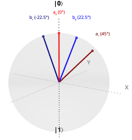
Bloch Sphere (3D and 2D): The geometric arrangement of measurement angles. Note the symmetry of the configuration: $b_0$ (22.5°) is positioned exactly halfway between $a_0$ (0°) and $a_1$ (45°), while $b_1$ (-22.5°) is symmetric with respect to the origin.
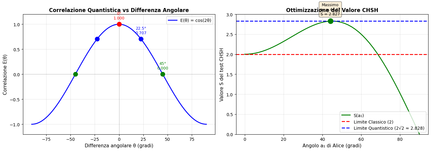
- Correlation vs Angular Difference: Shows how quantum correlation $E(\theta) = \cos(2\theta)$ depends on angular difference. CHSH angles are chosen to obtain specific correlation values that maximize S.
- CHSH value optimization: Visually demonstrates that the configuration with $a_1 = 45°$ (and consequently $b_0 = 22.5°$ , $b_1 = -22.5°$ ) effectively maximizes the violation of Bell’s inequalities.
In the CHSH experiment, measurement directions are symmetrically arranged to maximally exploit quantum correlations allowed by entanglement, exceeding the classical limit of 2 and reaching Tsirelson’s bound of $2\sqrt{2}$ .
6.6. What does this result mean?
Bell inequality violation tells us that:
There cannot exist a description of the physical world that satisfies the principles of locality and realism.
In other words:
- Either “actions at a distance” exist that allow entangled particles to “communicate” instantaneously (violation of locality)
- Or physical properties don’t exist before measurement but are created by the act of observation itself (violation of realism)
Most physicists today accept the interpretation that it’s realism that’s violated, while locality is preserved (although in a subtle way).
6.7. Other interactive experiments
Now that we’ve seen the basic CHSH test, let’s explore some additional experiments that help us better understand Bell inequality violation and the differences between quantum mechanics and local realism.
6.7.1. Variation of CHSH value with angles
This experiment shows how the CHSH value varies as Alice’s angle $a_1$ varies, keeping other angles fixed. It allows us to graphically see why 45° is the optimal angle.
import numpy as np
import matplotlib.pyplot as plt
from qiskit import QuantumCircuit, transpile
from qiskit_aer import AerSimulator

def compute_chsh_value(a0, a1, b0, b1, shots=8192):
    """Calculate CHSH value for a given angle configuration"""

    def compute_correlation(theta_a, theta_b):
        qc = QuantumCircuit(2, 2)
        qc.h(0)
        qc.cx(0, 1)
        qc.ry(2 * theta_a, 0)
        qc.ry(2 * theta_b, 1)
        qc.measure([0, 1], [0, 1])

        simulator = AerSimulator()
        compiled_circuit = transpile(qc, simulator)
        result = simulator.run(compiled_circuit, shots=shots).result()
        counts = result.get_counts()

        correlation = 0
        for outcome, count in counts.items():
            parity = 1 if outcome[0] == outcome[1] else -1
            correlation += parity * count / shots

        return correlation

    E_a0_b0 = compute_correlation(a0, b0)
    E_a0_b1 = compute_correlation(a0, b1)
    E_a1_b0 = compute_correlation(a1, b0)
    E_a1_b1 = compute_correlation(a1, b1)

    S = E_a0_b0 + E_a0_b1 + E_a1_b0 - E_a1_b1

    return S, (E_a0_b0, E_a0_b1, E_a1_b0, E_a1_b1)

# Vary angle a1 from 0 to 90 degrees
a1_values = np.linspace(0, np.pi/2, 20)
s_values_quantum = []
s_values_classical = 2 * np.ones_like(a1_values)  # Classical limit

print("Calculating CHSH values for different angles...")
for a1 in a1_values:
    # Fixed angles
    a0 = 0
    b0 = a1 / 2  # Optimal: halfway between a0 and a1
    b1 = -a1 / 2  # Symmetric with respect to a0

    S, _ = compute_chsh_value(a0, a1, b0, b1, shots=4096)
    s_values_quantum.append(S)
    print(f"a1 = {np.degrees(a1):.1f}°, S = {S:.3f}")

# Graph
plt.figure(figsize=(12, 6))

plt.plot(np.degrees(a1_values), s_values_quantum, 'b-o',
         linewidth=2, markersize=6, label='Quantum Simulation')
plt.axhline(y=2, color='r', linestyle='--', linewidth=2,
            label='Classical Limit (|S| ≤ 2)')
plt.axhline(y=2*np.sqrt(2), color='g', linestyle='--', linewidth=2,
            label=f'Tsirelson Bound (2√2 ≈ {2*np.sqrt(2):.3f})')
plt.axvline(x=45, color='orange', linestyle=':', linewidth=2,
            label='Optimal angle (45°)')

plt.xlabel('Angle a₁ (degrees)', fontsize=12)
plt.ylabel('CHSH Value (S)', fontsize=12)
plt.title('Bell Inequality Violation as Angle Varies',
          fontsize=14, fontweight='bold')
plt.legend(fontsize=10)
plt.grid(True, alpha=0.3)
plt.ylim([0, 3])

plt.tight_layout()
plt.savefig('chsh_angle_variation.png', dpi=300, bbox_inches='tight')
plt.show()

print(f"\n{'='*50}")
print(f"Maximum violation at 45°: S ≈ {max(s_values_quantum):.3f}")
print(f"Theoretical limit: 2√2 ≈ {2*np.sqrt(2):.3f}")
print(f"{'='*50}")
Expected result: The graph shows that maximum violation occurs precisely at 45°, where S reaches about 2.828.
6.7.2. Quantum vs classical comparison: correlation heatmap
This experiment visualizes quantum and classical correlations as heatmaps, allowing us to clearly see the difference.
import numpy as np
import matplotlib.pyplot as plt
from qiskit import QuantumCircuit, transpile
from qiskit_aer import AerSimulator

def compute_quantum_correlation(theta_a, theta_b, shots=8192):
    """Calculate quantum correlation for two angles"""
    qc = QuantumCircuit(2, 2)
    qc.h(0)
    qc.cx(0, 1)
    qc.ry(2 * theta_a, 0)
    qc.ry(2 * theta_b, 1)
    qc.measure([0, 1], [0, 1])

    simulator = AerSimulator()
    compiled_circuit = transpile(qc, simulator)
    result = simulator.run(compiled_circuit, shots=shots).result()
    counts = result.get_counts()

    correlation = 0
    for outcome, count in counts.items():
        parity = 1 if outcome[0] == outcome[1] else -1
        correlation += parity * count / shots

    return correlation

def compute_classical_correlation(theta_diff):
    """
    Maximum classical correlation possible for an angular difference.
    With local hidden variables, maximum correlation is limited.
    """
    # Classical model: linearly decreasing correlation
    return 1 - 2 * abs(theta_diff) / (np.pi/2)

# Angle grid
angles = np.linspace(0, np.pi/2, 12)
angles_deg = np.degrees(angles)

# Matrices for correlations
quantum_corr = np.zeros((len(angles), len(angles)))
classical_corr = np.zeros((len(angles), len(angles)))

print("Calculating quantum and classical correlations...")
for i, theta_a in enumerate(angles):
    for j, theta_b in enumerate(angles):
        # Quantum correlation
        quantum_corr[i, j] = compute_quantum_correlation(theta_a, theta_b, shots=2048)

        # Theoretical classical correlation
        theta_diff = abs(theta_a - theta_b)
        classical_corr[i, j] = compute_classical_correlation(theta_diff)

    print(f"Progress: {i+1}/{len(angles)}")

# Visualization
fig, (ax1, ax2, ax3) = plt.subplots(1, 3, figsize=(18, 5))

# Quantum heatmap
im1 = ax1.imshow(quantum_corr, cmap='RdBu_r', aspect='auto',
                 vmin=-1, vmax=1, origin='lower')
ax1.set_xlabel('Bob Angle (degrees)', fontsize=11)
ax1.set_ylabel('Alice Angle (degrees)', fontsize=11)
ax1.set_title('Quantum Correlations\n(Simulation)',
              fontsize=12, fontweight='bold')
ax1.set_xticks(range(len(angles_deg)))
ax1.set_yticks(range(len(angles_deg)))
ax1.set_xticklabels([f'{a:.0f}' for a in angles_deg], rotation=45)
ax1.set_yticklabels([f'{a:.0f}' for a in angles_deg])
plt.colorbar(im1, ax=ax1, label='Correlation E(a,b)')

# Classical heatmap
im2 = ax2.imshow(classical_corr, cmap='RdBu_r', aspect='auto',
                 vmin=-1, vmax=1, origin='lower')
ax2.set_xlabel('Bob Angle (degrees)', fontsize=11)
ax2.set_ylabel('Alice Angle (degrees)', fontsize=11)
ax2.set_title('Classical Correlations\n(Local Hidden Variables)',
              fontsize=12, fontweight='bold')
ax2.set_xticks(range(len(angles_deg)))
ax2.set_yticks(range(len(angles_deg)))
ax2.set_xticklabels([f'{a:.0f}' for a in angles_deg], rotation=45)
ax2.set_yticklabels([f'{a:.0f}' for a in angles_deg])
plt.colorbar(im2, ax=ax2, label='Correlation E(a,b)')

# Difference
difference = quantum_corr - classical_corr
im3 = ax3.imshow(difference, cmap='seismic', aspect='auto',
                 vmin=-0.5, vmax=0.5, origin='lower')
ax3.set_xlabel('Bob Angle (degrees)', fontsize=11)
ax3.set_ylabel('Alice Angle (degrees)', fontsize=11)
ax3.set_title('Difference\n(Quantum - Classical)',
              fontsize=12, fontweight='bold')
ax3.set_xticks(range(len(angles_deg)))
ax3.set_yticks(range(len(angles_deg)))
ax3.set_xticklabels([f'{a:.0f}' for a in angles_deg], rotation=45)
ax3.set_yticklabels([f'{a:.0f}' for a in angles_deg])
plt.colorbar(im3, ax=ax3, label='Difference')

plt.tight_layout()
plt.savefig('correlation_heatmaps.png', dpi=300, bbox_inches='tight')
plt.show()

print("\nRed zones in the difference map show where")
print("quantum correlations exceed classical ones!")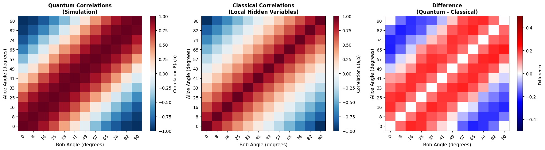 Interpretation: The heatmaps show how quantum correlations (which follow $\cos(2\theta)$
) differ significantly from classical ones, especially for intermediate angles.
Interpretation: The heatmaps show how quantum correlations (which follow $\cos(2\theta)$
) differ significantly from classical ones, especially for intermediate angles.
6.7.3. Interactive exploration of CHSH parameters
This experiment creates a complete parametric analysis of the CHSH angle space.
import numpy as np
import matplotlib.pyplot as plt
from matplotlib.widgets import Slider
from qiskit import QuantumCircuit, transpile
from qiskit_aer import AerSimulator

def compute_single_correlation(theta_a, theta_b, shots=4096):
    """Calculate a single correlation"""
    qc = QuantumCircuit(2, 2)
    qc.h(0)
    qc.cx(0, 1)
    qc.ry(2 * theta_a, 0)
    qc.ry(2 * theta_b, 1)
    qc.measure([0, 1], [0, 1])

    simulator = AerSimulator()
    compiled_circuit = transpile(qc, simulator)
    result = simulator.run(compiled_circuit, shots=shots).result()
    counts = result.get_counts()

    correlation = 0
    for outcome, count in counts.items():
        parity = 1 if outcome[0] == outcome[1] else -1
        correlation += parity * count / shots

    return correlation

# 2D analysis: simultaneous variation of a1 and b0
a1_range = np.linspace(0, np.pi/2, 25)
b0_range = np.linspace(0, np.pi/2, 25)

S_matrix = np.zeros((len(a1_range), len(b0_range)))

print("Exploring CHSH parameter space...")
print("This may take a few minutes...\n")

for i, a1 in enumerate(a1_range):
    for j, b0 in enumerate(b0_range):
        a0 = 0
        b1 = -b0

        E_a0_b0 = compute_single_correlation(a0, b0, shots=2048)
        E_a0_b1 = compute_single_correlation(a0, b1, shots=2048)
        E_a1_b0 = compute_single_correlation(a1, b0, shots=2048)
        E_a1_b1 = compute_single_correlation(a1, b1, shots=2048)

        S = E_a0_b0 + E_a0_b1 + E_a1_b0 - E_a1_b1
        S_matrix[i, j] = S

    if (i + 1) % 5 == 0:
        print(f"Progress: {i+1}/{len(a1_range)}")

# 3D visualization
fig = plt.figure(figsize=(16, 6))

# Subplot 1: 2D Heatmap
ax1 = fig.add_subplot(121)
im = ax1.contourf(np.degrees(b0_range), np.degrees(a1_range), S_matrix,
                  levels=20, cmap='RdYlGn')
ax1.contour(np.degrees(b0_range), np.degrees(a1_range), S_matrix,
            levels=[2.0], colors='red', linewidths=3,
            linestyles='--')
ax1.plot(22.5, 45, 'b*', markersize=20, label='Optimal configuration')
ax1.set_xlabel('Angle b₀ (degrees)', fontsize=12)
ax1.set_ylabel('Angle a₁ (degrees)', fontsize=12)
ax1.set_title('CHSH Value in Parameter Space',
              fontsize=13, fontweight='bold')
ax1.legend(fontsize=10)
ax1.grid(True, alpha=0.3)
cbar = plt.colorbar(im, ax=ax1, label='S')
cbar.ax.axhline(y=2, color='red', linewidth=2, linestyle='--')
cbar.ax.text(1.5, 2, 'Classical limit', rotation=0, va='center', fontsize=9)

# Subplot 2: 3D Surface
ax2 = fig.add_subplot(122, projection='3d')
B0, A1 = np.meshgrid(np.degrees(b0_range), np.degrees(a1_range))
surf = ax2.plot_surface(B0, A1, S_matrix, cmap='RdYlGn',
                        alpha=0.9, edgecolor='none')

# Classical limit plane
xx, yy = np.meshgrid(np.degrees(b0_range), np.degrees(a1_range))
zz = 2 * np.ones_like(xx)
ax2.plot_surface(xx, yy, zz, alpha=0.3, color='red')

ax2.set_xlabel('Angle b₀ (degrees)', fontsize=10)
ax2.set_ylabel('Angle a₁ (degrees)', fontsize=10)
ax2.set_zlabel('CHSH Value (S)', fontsize=10)
ax2.set_title('3D CHSH Surface', fontsize=13, fontweight='bold')
ax2.view_init(elev=25, azim=45)

fig.colorbar(surf, ax=ax2, shrink=0.5, aspect=5, label='S')

plt.tight_layout()
plt.savefig('chsh_parameter_space.png', dpi=300, bbox_inches='tight')
plt.show()

# Find maximum
max_idx = np.unravel_index(np.argmax(S_matrix), S_matrix.shape)
max_a1 = np.degrees(a1_range[max_idx[0]])
max_b0 = np.degrees(b0_range[max_idx[1]])
max_S = S_matrix[max_idx]

print(f"\n{'='*50}")
print(f"Optimal configuration found:")
print(f"  a₁ = {max_a1:.1f}°")
print(f"  b₀ = {max_b0:.1f}°")
print(f"  S = {max_S:.3f}")
print(f"\nOptimal theoretical value: a₁=45°, b₀=22.5°, S=2√2≈2.828")
print(f"{'='*50}")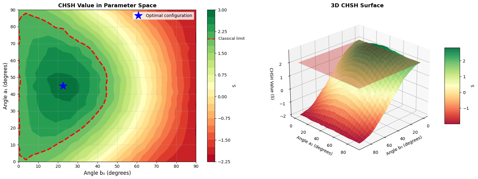 Result: This graph shows the “mountain” of the CHSH value in parameter space, with the peak precisely at the optimal configuration (45°, 22.5°).
6.7.4. Simulation with realistic noise
In the last experiment, we add noise to simulate imperfections of real quantum computers.
import numpy as np
import matplotlib.pyplot as plt
from qiskit import QuantumCircuit, transpile
from qiskit_aer import AerSimulator
from qiskit_aer.noise import NoiseModel, depolarizing_error, thermal_relaxation_error

def create_noisy_simulator(error_rate=0.01, t1=50, t2=70):
    """
    Create a simulator with realistic noise.

    Args:
        error_rate: probability of error per gate (depolarizing)
        t1: relaxation time T1 (microseconds)
        t2: decoherence time T2 (microseconds)
    """
    noise_model = NoiseModel()

    # Depolarizing error on gates
    error_gate1 = depolarizing_error(error_rate, 1)
    error_gate2 = depolarizing_error(error_rate * 2, 2)

    # Add errors to gates
    noise_model.add_all_qubit_quantum_error(error_gate1, ['h', 'ry'])
    noise_model.add_all_qubit_quantum_error(error_gate2, ['cx'])

    # Thermal relaxation error
    # gate_times = {'h': 50, 'ry': 50, 'cx': 200, 'measure': 1000}  # in nanoseconds
    # thermal_error = thermal_relaxation_error(t1*1000, t2*1000, gate_times['cx'])
    # noise_model.add_all_qubit_quantum_error(thermal_error, ['cx'])

    return noise_model

def run_chsh_with_noise(error_rate, shots=8192):
    """Execute CHSH test with a given noise level"""

    noise_model = create_noisy_simulator(error_rate=error_rate)
    simulator = AerSimulator(noise_model=noise_model)

    # Optimal angles
    a0, a1 = 0, np.pi/4
    b0, b1 = np.pi/8, -np.pi/8

    def compute_correlation(theta_a, theta_b):
        qc = QuantumCircuit(2, 2)
        qc.h(0)
        qc.cx(0, 1)
        qc.ry(2 * theta_a, 0)
        qc.ry(2 * theta_b, 1)
        qc.measure([0, 1], [0, 1])

        compiled_circuit = transpile(qc, simulator)
        result = simulator.run(compiled_circuit, shots=shots).result()
        counts = result.get_counts()

        correlation = 0
        for outcome, count in counts.items():
            parity = 1 if outcome[0] == outcome[1] else -1
            correlation += parity * count / shots

        return correlation

    E_a0_b0 = compute_correlation(a0, b0)
    E_a0_b1 = compute_correlation(a0, b1)
    E_a1_b0 = compute_correlation(a1, b0)
    E_a1_b1 = compute_correlation(a1, b1)

    S = E_a0_b0 + E_a0_b1 + E_a1_b0 - E_a1_b1

    return S, (E_a0_b0, E_a0_b1, E_a1_b0, E_a1_b1)

# Test with different noise levels
error_rates = np.linspace(0, 0.10, 20)
s_values_noisy = []
s_std = []

print("Simulation with realistic noise...")
print("This simulates imperfections of real quantum computers.\n")

for error_rate in error_rates:
    # Run multiple times to estimate variance
    s_trials = []
    for _ in range(5):
        S, _ = run_chsh_with_noise(error_rate, shots=4096)
        s_trials.append(S)

    s_values_noisy.append(np.mean(s_trials))
    s_std.append(np.std(s_trials))

    print(f"Error rate: {error_rate*100:.1f}% → S = {np.mean(s_trials):.3f} ± {np.std(s_trials):.3f}")

# Visualization
fig, (ax1, ax2) = plt.subplots(1, 2, figsize=(16, 6))

# Subplot 1: S vs Error Rate
s_values_noisy = np.array(s_values_noisy)
s_std = np.array(s_std)

ax1.errorbar(error_rates * 100, s_values_noisy, yerr=s_std,
             fmt='o-', linewidth=2, markersize=8, capsize=5,
             color='blue', label='Simulation with noise')
ax1.axhline(y=2, color='red', linestyle='--', linewidth=2,
            label='Classical limit (S=2)')
ax1.axhline(y=2*np.sqrt(2), color='green', linestyle='--', linewidth=2,
            label=f'Ideal limit (S=2√2≈{2*np.sqrt(2):.3f})')
ax1.fill_between(error_rates * 100, 2, s_values_noisy,
                 where=(s_values_noisy > 2), alpha=0.3, color='green',
                 label='Violation zone')

ax1.set_xlabel('Error rate per gate (%)', fontsize=12)
ax1.set_ylabel('CHSH Value (S)', fontsize=12)
ax1.set_title('Effect of Noise on Bell Violation',
              fontsize=13, fontweight='bold')
ax1.legend(fontsize=10)
ax1.grid(True, alpha=0.3)
ax1.set_ylim([1.5, 3])

# Subplot 2: Violation vs Error Rate
violation = s_values_noisy - 2
ax2.bar(error_rates * 100, violation, width=0.25,
        color=['green' if v > 0 else 'red' for v in violation],
        alpha=0.7, edgecolor='black')
ax2.axhline(y=0, color='black', linestyle='-', linewidth=1)
ax2.set_xlabel('Error rate per gate (%)', fontsize=12)
ax2.set_ylabel('Violation (S - 2)', fontsize=12)
ax2.set_title('Margin of Bell Inequality Violation',
              fontsize=13, fontweight='bold')
ax2.grid(True, alpha=0.3, axis='y')

# Find critical point where S drops below 2
critical_idx = np.where(s_values_noisy < 2)[0]
if len(critical_idx) > 0:
    critical_error = error_rates[critical_idx[0]] * 100
    ax2.axvline(x=critical_error, color='red', linestyle=':', linewidth=2)
    ax2.text(critical_error, ax2.get_ylim()[1] * 0.8,
             f'Critical point\n~{critical_error:.1f}%',
             ha='center', fontsize=10, bbox=dict(boxstyle='round',
             facecolor='wheat', alpha=0.5))

plt.tight_layout()
plt.savefig('chsh_with_noise.png', dpi=300, bbox_inches='tight')
plt.show()

print(f"\n{'='*60}")
print("RESULTS:")
print(f"  - With 0% noise: S ≈ {s_values_noisy[0]:.3f} (ideal)")
print(f"  - With 1% noise: S ≈ {s_values_noisy[int(len(s_values_noisy)*0.2)]:.3f}")
print(f"  - With 3% noise: S ≈ {s_values_noisy[int(len(s_values_noisy)*0.6)]:.3f}")
if len(critical_idx) > 0:
    print(f"  - Critical limit: ~{critical_error:.1f}% (S drops below 2)")
else:
    print(f"  - Violation persists up to {error_rates[-1]*100:.1f}%")
print(f"{'='*60}")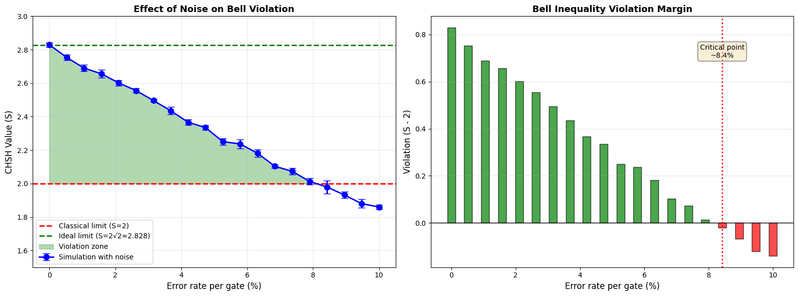 Interpretation: This graph shows how delicate quantum computers are. Even small errors reduce Bell violation, but fortunately it takes a fairly high error (>8%) before the violation completely disappears.
7. Conclusions and philosophical reflections
7.1. Who was right?
The Einstein-Bohr debate was one of the most fascinating in the history of physics. From a purely scientific point of view, we can say that Bohr was right: quantum mechanics is a complete and correct theory, and quantum phenomena cannot be explained with local hidden variable theories.
Einstein’s fate was somewhat paradoxical: despite being recognized as one of the greatest physicists of all time, he was often misunderstood and isolated by the “mainstream” scientific community, both in the early phases of his career (with relativity) and in the final ones (with quantum mechanics).
In any case, I believe that the very formulation of the EPR problem, which then led to Bell’s studies, Aspect’s experiments, and those of many others, was once again an enormous contribution to physics and human knowledge.
7.2. The nature of reality
From a philosophical point of view, Bell’s experiments teach us something profound about the nature of reality:
- The world is not made of “things” with defined properties that exist independently of observation
- Reality emerges from interaction between observed system and measurement apparatus
- We cannot completely separate the observer from the observed
This doesn’t mean that reality “doesn’t exist” or that it’s purely subjective, but rather that our classical intuition about what it means to “exist” must be profoundly revised in light of quantum phenomena.
In a certain sense, what we identify as “reality” is an emergent construct and doesn’t transcend our interactions with the world.